Your second Machine Learning Project with this famous IRIS dataset in python (Part 5 of 6)
We have successfully completed our first project to predict the salary, if you haven't completed it yet, click here to finish that tutorial first.
Our first project was simple supervised learning project based on regression. We can now go ahead and create a project based on a classification algorithm.
Steps involved in a machine learning project:
Following are the steps involved in creating a well-defined ML project:
- Understand and define the problem
- Analyse and prepare the data
- Apply the algorithms
- Reduce the errors
- Predict the result
Our second Project : Lets predict the species of a flower based on the petal width and size
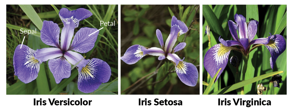
The IRIS flower data set contains the the physical parameters of three species of flower — Versicolor, Setosa and Virginica. The numeric parameters which the dataset contains are Sepal width, Sepal length, Petal width and Petal length. In this data we will be predicting the species of the flowers based on these parameters. We will be building a machine learning project to determine the species of the flower.
Please note this is not a image-classifier algorithm, We are only feeding the measurements to the algorithm in number format (for simplicity purposes)
Load the salaries data set
- Launch Anaconda navigator and open the terminal
- Type the below command to start the python environment
python
- Lets make sure the python environment is up and running. Copy paste the below command in the terminal to check if its working properly
print("Hello World")- Nice and clear, we are all set to write our program. First its important that we import all the required libraries for our project. So copy-paste the below commands into the terminal. (You can copy all of them at once)
#Load libraries
import pandas as pd
import numpy as np
import matplotlib.pyplot as plt
from sklearn import model_selection
from sklearn.metrics import accuracy_score
from sklearn.linear_model import LogisticRegression
from sklearn.linear_model import LinearRegression
from sklearn.ensemble import RandomForestClassifier
from sklearn.neighbors import KNeighborsClassifier
from sklearn.svm import SVC
- Lets load the IRIS flowers training data set and assign it to a variable called "dataset". We are using pandas to load the data. We will also use pandas next to explore the data both with descriptive statistics and data visualization
#Load dataset
url = "https://raw.githubusercontent.com/callxpert/datasets/master/iris.data.txt"
names = ['sepal-length', 'sepal-width', 'petal-length', 'petal-width', 'class']
dataset = pd.read_csv(url, names=names)
Summarize the data and perform analysis
Lets take a peek into our training data set:
- Dimensions of data set: Find out how many rows and columns our dataset has using the shape property
# shape
print(dataset.shape)
Result: (150,5), Which means our dataset has 150 rows and 5 columns
- To see the first 20 rows of our dataset
print(dataset.head(20))
Result:
    sepal-length  sepal-width  petal-length  petal-width        class
0            5.1          3.5           1.4          0.2  Iris-setosa
1            4.9          3.0           1.4          0.2  Iris-setosa
2            4.7          3.2           1.3          0.2  Iris-setosa
3            4.6          3.1           1.5          0.2  Iris-setosa
4            5.0          3.6           1.4          0.2  Iris-setosa
5            5.4          3.9           1.7          0.4  Iris-setosa
6            4.6          3.4           1.4          0.3  Iris-setosa
7            5.0          3.4           1.5          0.2  Iris-setosa
8            4.4          2.9           1.4          0.2  Iris-setosa
9            4.9          3.1           1.5          0.1  Iris-setosa
10           5.4          3.7           1.5          0.2  Iris-setosa
11           4.8          3.4           1.6          0.2  Iris-setosa
12           4.8          3.0           1.4          0.1  Iris-setosa
13           4.3          3.0           1.1          0.1  Iris-setosa
14           5.8          4.0           1.2          0.2  Iris-setosa
15           5.7          4.4           1.5          0.4  Iris-setosa
16           5.4          3.9           1.3          0.4  Iris-setosa
17           5.1          3.5           1.4          0.3  Iris-setosa
18           5.7          3.8           1.7          0.3  Iris-setosa
19           5.1          3.8           1.5          0.3  Iris-setosa
- Find out the statistical summary of the data including the count, mean, the min and max values as well as some percentiles.
print(dataset.describe())
Result:
       sepal-length  sepal-width  petal-length  petal-width
count    150.000000   150.000000    150.000000   150.000000
mean       5.843333     3.054000      3.758667     1.198667
std        0.828066     0.433594      1.764420     0.763161
min        4.300000     2.000000      1.000000     0.100000
25%        5.100000     2.800000      1.600000     0.300000
50%        5.800000     3.000000      4.350000     1.300000
75%        6.400000     3.300000      5.100000     1.800000
max        7.900000     4.400000      6.900000     2.500000
- Lets find the class distribution of the dataset
#class distribution
print(dataset.groupby('class').size())
Result:
class
Iris-setosa        50
Iris-versicolor    50
Iris-virginica     50
dtype: int64
Which implies our dataset has an even distribution of 50 records for each species type.
Analysing the data visually
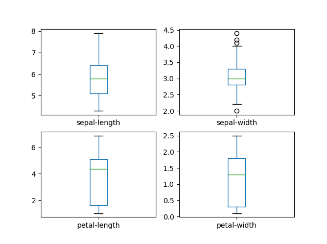
- Let us create a box plot of the dataset, it will show us the visual representation of how our data is scattered over the the plane. Box plot is a percentile-based graph, which divides the data into four quartiles of 25% each. This method is used in statistical analysis to understand various measures such as mean, median and deviation
# box and whisker plots
dataset.plot(kind='box', subplots=True, layout=(2,2), sharex=False, sharey=False)
plt.show()
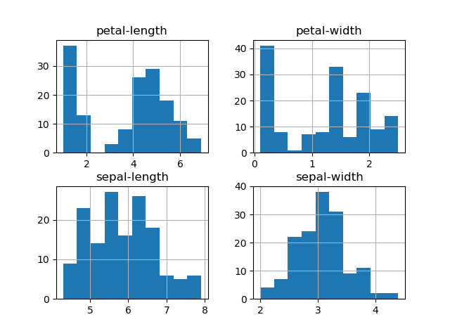
- We can also create a histogram of each input variable to get an idea of the distribution.
# histograms
dataset.hist()
plt.show()
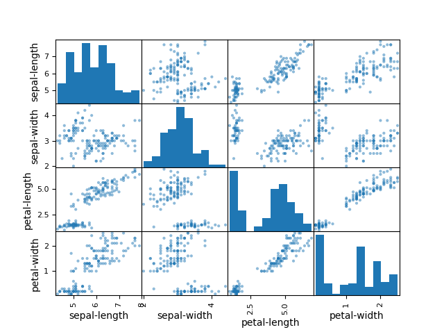
- To understand how each feature for classification of the data, we can build a scatter plot which shows us the correlation with respect to other features. This method helps just to figure out the important features which account the most for the classification in our model
# scatter plot matrix
from pandas.plotting import scatter_matrix\nscatter_matrix(dataset)
plt.show()
Splitting the Data
As we have seen already, In Machine learning we have two kinds of datasets
- Training dataset - used to train our model
- Testing dataset - used to test if our model is making accurate predictions
Since our dataset is small (150 records) we will use 120 records for training the model and 30 records to evaluate the model. copy paste the below commands to prepare our datasets
array = dataset.values
X = array[:,0:4]
Y = array[:,4]
x_train, x_test, y_train, y_test = model_selection.train_test_split(X, Y, test_size=0.2, random_state=7)
Evaluating the model and training the Model
We are going to apply the below four algorithms to this problem and evaluate its effectiveness. And finally choose the best algorithm and train it.
- K – Nearest Neighbour (KNN)
- Support Vector Machine (SVM)
- Randomforest
- Logistic Regression
Lets apply the KNN Algorithm and train the model and predict the accuracy with our testing dataset.
model = KNeighborsClassifier()
model.fit(x_train,y_train)
predictions = model.predict(x_test)
print(accuracy_score(y_test, predictions))
Result: 0.9
Next, lets test the Support Vector Machine model works on the principle of Radial Basis function with default parameters
model = SVC()
model.fit(x_train,y_train)
predictions = model.predict(x_test)
print(accuracy_score(y_test, predictions))
Result: 0.9333333333333333
Let us try the third one in our list. Randomforest is one of the highly accurate nonlinear algorithm, which works on the principle of Decision Tree Classification
model = RandomForestClassifier(n_estimators=5)
model.fit(x_train,y_train)
predictions = model.predict(x_test)
print(accuracy_score(y_test, predictions))
Result: 0.8666666666666667
Let us try the the last algorithm from our list. The Logistic Regression:
model = LogisticRegression()
model.fit(x_train,y_train)
predictions = model.predict(x_test)
print(accuracy_score(y_test, predictions))
Result: 0.8
Please note: Your accuracy score may vary as we have chosen to randomly pick our test data.
From the score, we can infer that SVG algorithm is very effective among the four. Our dataset is small, so we need to get more examples / training data to find out an effective algorithm that works for our use case.
Summary
In ML, there is no specific model or an algorithm which can give 100% result to every single dataset. In this post, you have discovered step-by-step on how to create and train a model using supervised classification algorithm
Next step: Your third practice project in machine learning with python
Share your thought in the comments. And share your knowledge with others in the copycoding community
nVector
posted onEnjoy great content like this and a lot more !
Signup for a free account to write a post / comment / upvote posts. Its simple and takes less than 5 seconds
Post Comment